Warning: This article is extremely long
Hello readers, welcome to the “Kaoprao” article series! Just reading the title, you might wonder what on earth this series is actually about. Let me preface this first: whether back in our hometowns or out in the countryside, rice is our staple food. But living in the concrete jungle of the big city, how many of us actually cook rice at home anymore?
Of course, you European/Murican might not get this since the native rice-based product there is “Bread”. That basically the same thing.
The “Kaoprao” series is just like that. Think of it like cooking rice from scratch (or bread from scratch idk). What do we have to do before cooking? Rinse the rice? Rake the grains? Who cares… The point is, “Kaoprao” is all about taking readers down the rabbit hole of software architecture, uncovering process behind the tools we use daily. That is “Kaoprao”.
In today’s Kaoprao, I’m sure most of you use or have used note-taking apps. Especially if you own a Tablet/iPad, it’s pretty much a must-have (because default built-in OS note apps are notoriously) terrible. So we rely on third-party apps like Goodnotes, Freenotes, Element Note, Notability, and so on.
And I bet many of you pay subscription fees for these apps in exchange for convenience at school or work. But under all that convenience, have you ever wondered how the stack inside actually works under the hood to feel so buttery smooth (not counting default iOS ones)? Today, we’re cracking it open, and our main target today is Freenotes.
So what are we dissecting first? If you’ve ever exported notes from these apps, besides standard .pdf or .png files, you’ve probably seen proprietary formats like .freenotes or .goodnotes that can only be opened within those specific apps. Unlike other formats, these proprietary files store data losslessly, meaning anyone who downloads or recovers the file can open and continue editing it seamlessly.
Before We Begin
First, we need to understand that even though the file has a .freenotes extension, internally it is actually a Zip archive. If we download the file and inspect it, we’ll find that it’s just a Zip file.
<xxxx>.freenotes: Zip archive data, made by v3.0 UNIX, extract using at least v4.5, last modified YYYY, method=deflateIn the next section, we’ll dive into the detailed file structure. In this article, our main focus will be on the .freenotes format.
File Structure
Before diving deep, let’s extract the file to examine its structure and plan our next steps.
Once extracted, we find the following file structure:
[BOX] .frnote File Structure [ CLICK TO UNBOX ] [ CLICK TO CLOSE ]
915CB187-E62E-439E-AD9B-DC50DA3AAC13.frnote/
├── AssetState
│   ├── imageObjectState.dat
│   ├── imageState.dat
│   └── pdfState.dat
├── document.dat
├── FNPages
│   └── 3C892967-BC80-4C5F-B384-FB2045DEC9CA.dat
├── FNPagesObject
├── FNPagesSummary
│   └── 3C892967-BC80-4C5F-B384-FB2045DEC9CA.dat
├── Images
├── index.db
├── layerInfo.dat
├── layout.dat
├── metadata.dat
├── Objects
│   └── Images
├── OCRRequests
│   └── requests.dat
├── OCR_v3
│   └── en-US
│       └── D0E31896-FAE8-460B-A9F8-69909A199688
│           ├── content.dat
│           └── summary.dat
├── PDFs
│   ├── 2F8DA175-4F19-4ADA-9FD2-B2369CE08F77.pdf
│   └── idMap.dat
├── Records
│   └── record.dat
├── Thumbnail
│   ├── Dark
│   │   └── Cover
│   │       ├── 775251DC-90E3-4C40-8B98-912ED498456F.png
│   │       └── Data.dat
│   └── Light
│       └── Cover
│           ├── 20696BD2-BF7E-417B-A75D-70A079CB82DE.png
│           └── Data.dat
├── versionList.dat
└── WebVideos
    └── webVideo.dat
Protobuf
Once extracted, what we get is a massive number of files that we have no idea how to read (if given to AI, it knows it’s Protobuf 😂, but we won’t take the easy way out). We start by exploring the file byte by byte, using metadata.dat as an example.
00000000  0a 24 39 31 35 43 42 31  38 37 2d 45 36 32 45 2d    |.$915CB187-E62E-|
00000010  34 33 39 45 2d 41 44 39 42 2d 44 43 35 30 44 41       |439E-AD9B-DC50DA|
00000020  33 41 41 43 31 33 1a 08  61 72 74 69 63 6c 65 77    |3AAC13..articlew|
Tag Length Value
First, it’s important to understand that Protobuf payloads work somewhat differently from other protocols: there is no Magic Code, making them slightly harder to identify than other protocols. However, they still have a distinct characteristic—each payload consists of 3 parts: Tag, Length, Value
Tag
The Tag acts like a label for each payload, consisting of 2 parts:
- Field Number (the data field number)
- Wire Type (the data type)
Suppose our data is 0x0A, which converts from HEX -> Binary as 0b00001010, and we can decode it as follows:
00001 | 010
 ^^^^^     ^^^
 Field     Wire Type
We can decode the information further:
- Field
00001->1:- Field Number equals 1
- Wire Type
010->2:- Wire Type = 2 corresponds to ‘Length-delimited’ (a payload without a fixed length), meaning the next byte must specify the payload length, or
LEN
- Wire Type = 2 corresponds to ‘Length-delimited’ (a payload without a fixed length), meaning the next byte must specify the payload length, or
Length (Optional)
Length or LEN is a component that may or may not be present, but is used for payloads that are not fixed in length.
In this case, 0x24 = 36, which means we need to read the next 36 Bytes.
Value
For variable-length payloads, this section contains the actual data content. In this case, it reads continuously for all 36 Bytes to the end.
Before Moving Forward
Now that we know this data (*.dat) is indeed Protobuf, the next step is decoding the Protobuf data. Normally, to read Protobuf, one must have a .proto schema file. Since we don’t have that schema, we will decode the raw data blindly without a guide. To read the data, we can use protoc like this:
protoc --decode_raw < metadata.dat[BOX] metadata.dat raw decoded [ CLICK TO UNBOX ] [ CLICK TO CLOSE ]
1: "915CB187-E62E-439E-AD9B-DC50DA3AAC13"
3: "articlew"
4: "articlew"
6 {
  1: 1785397999
  2: 484794140
}
8 {
  1: 1785398005
  2: 949923992
}
11: 0
Note:
articlewis the name of the notebook used for inspection, which was set manually and is not a default name from Freenotes.
Reverse Engineering Raw Files
In the previous section, we proved that all *.dat files are Protobuf files. However, we don’t know which Entity is which. How do we solve this?
Very simple.
Guess.
Not joking—since we don’t have a manual, the easiest approach is finding relationships between each file. From observation, we found:
Observations
- Each object has its own unique ID, which is a UUID.
- Each UUID maintains relationships linking back and forth according to
.datfilenames like Layout, Metadata, Document, etc. index.dbseems to store OCR data and Text objects, which is not our focus.
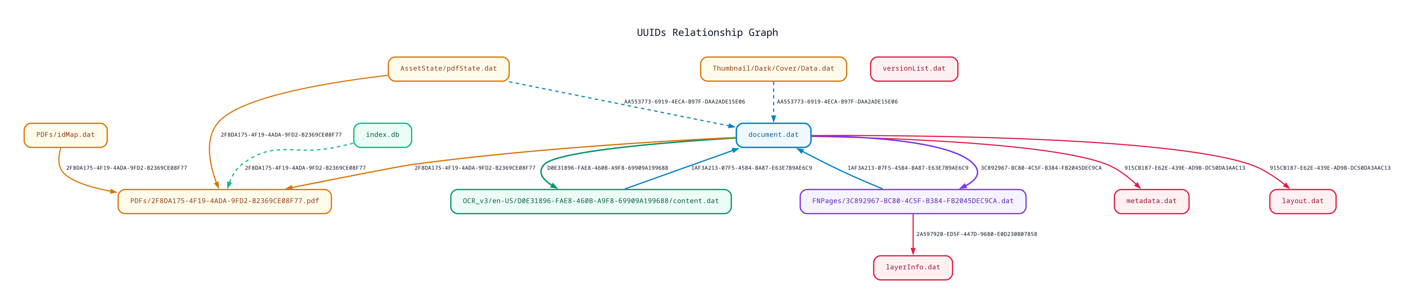
This might be hard to visualize—here is a basic relationship graph showing connections between various UUID values:
document.dat
From the graph, we found that each file is interconnected with document.dat acting as the central hub for all metadata. We began by decoding this file, highlighting the UUID connections across each document file in this set:
1: 2
2: "915CB187-E62E-439E-AD9B-DC50DA3AAC13" # Document UUID
4 {
  # Page Entry 1: Example linking PDF and Cover Page
  1 {
    1: "AA553773-6919-4ECA-B97F-DAA2ADE15E06" # Page UUID
    ...
    3 {
      2: "2F8DA175-4F19-4ADA-9FD2-B2369CE08F77" # REF: PDFs/<uuid>.pdf
    }
  }
  # Page Entry 2: Example linking Stroke (.dat) and OCR (.json)
  1 {
    1: "1AF3A213-07F5-45B4-BA87-E63E7B9AE6C9" # Page UUID
    6: "3C892967-BC80-4C5F-B384-FB2045DEC9CA" # REF: FNPages/<uuid>.dat
    8: "D0E31896-FAE8-460B-A9F8-69909A199688" # REF: OCR_v3/en-US/<uuid>/content.json
  }
}
(Note: View full raw dump in the Appendix)
Document_uuid Page_uuid Pdf_uuid FNPages_uuid OCR_uuid
Reading raw file structures of document.dat alone might make it difficult to understand Freenotes’ overall file structure.
Let’s look at an overview of document.dat to see how each component relates:
Document (Main note document / document.dat)
│
├── Metadata     (General metadata e.g. note title, creation date / metadata.dat)
├── Layout       (Paper size per page e.g. A4 / layout.dat)
├── Pages        (List of all pages in the document)
│      │
│      └── Stroke (Vector stroke coordinates per page / FNPages/<uuid>.dat)
│
└── PDF (Imported background PDF file / PDFs/<uuid>.pdf)FNPages/.dat
This is the most interesting file of all. Although at first glance it might seem unremarkable, looking closely reveals:
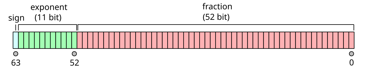
0x3ff0000000000000 is the IEEE-754 Hex Representation of double-precision floating-point numbers, or Double value equal to 1.0.
And it’s not just 1.0; there are floating-point values at multiple points throughout the file that indicate X, Y coordinates, making us confident that this file stores pen Strokes.
1: "3C892967-BC80-4C5F-B384-FB2045DEC9CA" # FNPages UUID
2: "1AF3A213-07F5-45B4-BA87-E63E7B9AE6C9" # Page UUID
3 {
  1: "54C99B69-BB82-4936-A855-9354BAE8C45B"
  2 {
    1 {
      1: "54C99B69-BB82-4936-A855-9354BAE8C45B"
      2 {
        1: 1                # Tool ID (1 = Ballpoint Pen)
        2: 2377619967       # #8DB799FF Color Hex
      }
      3 {
        1: 0x3ff0000000000000 # Scale X (double: 1.0)
        4: 0x3ff0000000000000 # Scale Y (double: 1.0)
      }
      4 {
        1: "2A59792B-ED5F-447D-9680-E0D230B07858" # Stroke Segment UUID
        # Touch Point 1
        2 {
          1 {
            1: 0x4064a0b4eb000000 # X (double: 165.022086)
            2: 0x4064a842f20b1378 # Y (double: 165.258172)
          }
          3 {
            1: 0x4002917f20000000 # Start Weight (double: 2.321045)
            2: 0x4002917f20000000 # End Weight (double: 2.321045)
          }
          4: 0xbf90647fe0000000 # Delta Time ($\Delta t = -0.016008$s)
        }
        # Touch Point 2
        2 {
          1 {
            1: 0x4064f20362e80000 # X (double: 167.562892)
            2: 0x4064b466bc170e50 # Y (double: 165.637540)
          }
          ...
        }
      }
    }
  }
}
(Note: View full raw dump in the Appendix)
Document_uuid Page_uuid Pdf_uuid FNPages_uuid OCR_uuid
PDFs/Layout.dat
This part might not seem like much, but if we convert 0x4082980000000000 and 0x408a500000000000 according to IEEE-754, we get 595 x 842, which in pts units is the standard size of an A4 layout. We can assume 3->1->[1-2] represent width and height.
1: "915CB187-E62E-439E-AD9B-DC50DA3AAC13" # Document UUID
2: 0x4082980000000000 # Document Width (double: 595.0 pt)
# Page Layout (Example 1 page):
3 {
  1 {
    1: 0x4082980000000000 # Width  (double: 595.0 pt)
    2: 0x408a4cf81852b2c6 # Height (double: 841.62 pt - Standard A4 size)
  }
  5: "AA553773-6919-4ECA-B97F-DAA2ADE15E06" # Page UUID
}
(Note: View full raw dump in the Appendix)
Document_uuid Page_uuid Pdf_uuid FNPages_uuid OCR_uuid
Others
Since the primary objective of this blog post is to dive deep into how vector drawing strokes are stored and processed,
if you are interested in viewing the full decoded data, you can check the Appendix at the bottom.
Computer Graphics Principles
In Computer Graphics, there are two main types of graphics: Raster Graphics and Vector Graphics:
-
Raster Graphics
-
Raster Graphics
- Images are created by coloring small rectangular pixels together to form the visible image.
- Lossy, meaning scaling may result in pixel loss.
- Primarily used today for computer displays, etc.
-
Vector Graphics
- Images are created by defining points and coordinates on a Cartesian coordinate system, consisting of points, curves, or geometric shapes.
- Lossless, meaning they can be scaled infinitely without quality loss.
- Cannot represent 100% photorealistic scenes.
If you’ve used standard drawing programs like Krita or IbisPaint, most default to Raster Graphics or file types like .png, .jpeg, .gif. Some applications allow switching layers to Vector, but that doesn’t mean everything is raster; files like .pdf are also Vector.
Looking from a System Analyst (SA) perspective when designing a handwriting note app—which mostly involves writing on blank templates (white A4, etc.) or imported PDF files—it needs to support:
- Lasso selection for moving objects
- Infinite scaling without losing data while maintaining smooth appearance
- Support for Undo/Redo
The simplest and most user-friendly approach is designing vector data storage. That is, instead of saving pixel-by-pixel, we store coordinates traced continuously before the pen is lifted, sampling at regular thresholds (Freenotes samples roughly every ~16ms). These are compiled into multiple vector lines layered on the canvas according to the pts dimensions set during creation, with $(0,0)$ typically starting at the top-left of the Cartesian coordinate system.
Building Strokes from Scratch
After decoding binary coordinates from FNPages/3C892967-BC80-4C5F-B384-FB2045DEC9CA.dat in the previous section, we can take the raw $(x, y)$ coordinates, Hex color (#8DB799FF), stroke width (2.321045 pt), and relative timestamp ($\Delta t$) of all 6 points to understand the step-by-step rendering process:
From the canvas, the coordinate details of the 6 Touch Event points are as follows:
- $P_0$ (Start Point): $(165.022, 165.258)$ | $\Delta t = -0.016008\text{ s}$
- $P_1$: $(167.563, 165.638)$ | $\Delta t = +0.004992\text{ s}$
- $P_2$: $(173.915, 166.528)$ | $\Delta t = +0.021992\text{ s}$
- $P_3$: $(182.461, 167.434)$ | $\Delta t = +0.037992\text{ s}$
- $P_4$: $(191.536, 167.749)$ | $\Delta t = +0.051000\text{ s}$
- $P_5$ (End Point): $(211.846, 166.677)$ | $\Delta t = +0.072000\text{ s}$
Curve Fitting for Vector Strokes
Now that we see the structure of the vectors we built, we notice that lines between points $P_i$ and $P_{i+1}$ are completely straight, stiff, and unnatural. What we are missing is generating smooth curves between points $P_i$ and $P_{i+1}$.
The fundamental Computer Graphics formula for this problem is the Bézier curve, starting with Linear Bézier:
$${B} (t)=(1-t) {p} _{0}+t {p} _{1}, t\in [0,1].$$From this formula, the segment between $P_i$ and $P_{i+1}$ remains a rigid straight line, lacking the natural curvature of real handwriting.
It only generates straight lines between two points.
Smoothing with Cubic Bézier (Degree 3)
To produce smooth curves, we use Cubic Bézier (Degree 3), adding control points P₁ and P₂:
$$ B(t) = (1-t)^3 P_0 + 3(1-t)^2 t P_1 + 3(1-t) t^2 P_2 + t^3 P_3 $$- \(P_0\) = Start point of the curve (Start Point)
- \(P_1\) = Control Point 1
- \(P_2\) = Control Point 2
- \(P_3\) = End point of the curve (End Point)
- \(t\) = Parameter where \(0 \le t \le 1\)
- \(B(t)\) = Point position on the curve for a given \(t\)
Ensuring $C^1$ Continuity
To prevent sharp kinks at join points, midpoints (Midpoint) must be calculated to keep curve transitions seamless:
$$ M_i = \frac{{P_i + P_{i+1}}}{2}$$Midpoint Calculation Example
- $P_0 = (0,0)$ (Start point)
- $P_1 = (4,8)$ (Current point)
- $P_2 = (12,4)$ (Next point)
Calculate midpoint $M_1$ between $P_1(4,8)$ and $P_2(12,4)$:
$$M_1 = \left( \frac{4+12}{2}, \frac{8+4}{2}\right) = (8,6)$$We obtain 4 control points for this curve:
- $C_0 = (0,0)$ [Start point]
- $C_1 = (4,8)$ [Control point 1: x1, y1]
- $C_2 = (8,6)$ [Control point 2: mid_x, mid_y]
- $C_3 = (8,6)$ [End point: mid_x, mid_y]
Substituting into the equation:
$$ B(t) = (1 - t)^{3}C_0 + 3(1 - t)^2tC_1 + 3(1 - t)t^2C_2 + t^3C_3 $$Substitute $C_i$ separately for $X, Y$ and set $t$ with the parameter, or:
# Draw degree-3 cubic Bezier curve to midpoint Mi
ctx.curve_to(x1, y1, mid_x, mid_y, mid_x, mid_y)
This command is automatically converted to the PDF Operator y / c (Curveto) in PDF files, yielding crisp vector handwriting with $C^1$ Continuity that doesn’t pixelate when zoomed in.
We aren’t done yet! If we have more than 3 points, we take $M_1 = (8,6)$ and proceed to calculate the next point. For example:
- $P_1 = (4,8)$ (Previous point)
- $P_2 = (12,4)$ (Current point)
- $P_3 = (20,10)$ (Next point)
This section might be a bit confusing… even the author got confused haha
You can learn more in 6.837: Introduction to Computer Graphics (fall 2020) by Justin Solomon
The Right Person Tool is Always Satisfying
In the previous section, we dived deep to revive our vector and add wings curves to it. Now that we’ve mastered the basics, the next step is applying this to more complex vectors.
As shown below:
At first glance, our graph might look beautiful and perfect… but wait! What you see might not be what it actually is. Believe it or not, we aren’t even close to the real thing yet :)
So that readers don’t feel like fighting with empty air, here is the actual screenshot fresh off the app:
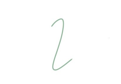
If we compare the actual screenshot with the graph above, we might notice a similarity—an inverted S-curve segment. If the black line (in the graph) represents our main stroke, what is everything else? That is what we will answer in the upcoming sections.
Ballpoint Pen
If we look back at our original file structure, we’ll find an interesting point. Namely this block:
2 {
  1: 1
  2: 2377619967         # #8DB799FF Color Hex
}
(Note: View full raw dump in the Appendix)
We find 2377619967, which converts to Hex as #8DB799FF—matching our pen color exactly.
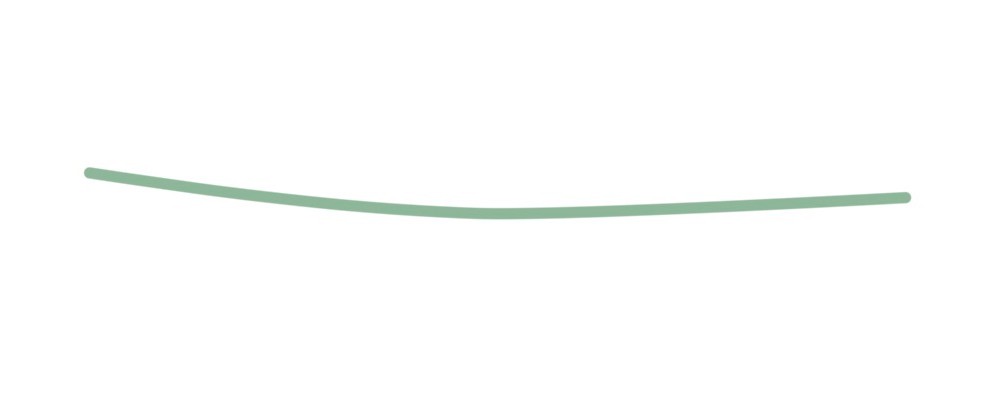
This confirms that this data block defines pen characteristics such as color and tip type.
Diving deeper into coordinates and stroke weights for the Ballpoint Pen, we find the following structure:
4 {
  1: "CBE801A9-59C1-4698-B9EC-61B12D3E0422"
  2 {
    1 {
      1: 0x4070da82b3c37a63 # (double: 269.6568865804606)
      2: 0x406886d5b4a4c882 # (double: 196.21308480620384)
    }
    3 {
      1: 0x4015d72cc0000000 # (double: 5.459999999999999)
      2: 0x4015d72cc0000000 # (double: 5.459999999999999)
    }
    4: 0xbf8c87e0c0000000 # (double: -0.013912320137023926)
  }
(Note: View full raw dump in the Appendix)
This is identical to the concept in this section.
Eraser
One of the most essential features in a note-taking/drawing app is the eraser, or the ability to remove unwanted portions from strokes.
From a user standpoint, erasing seems simple: drag over an area, and it disappears. Technologically, however, erasing is one of the most complex systems because behind that simple appearance lies intricate data organization and techniques.
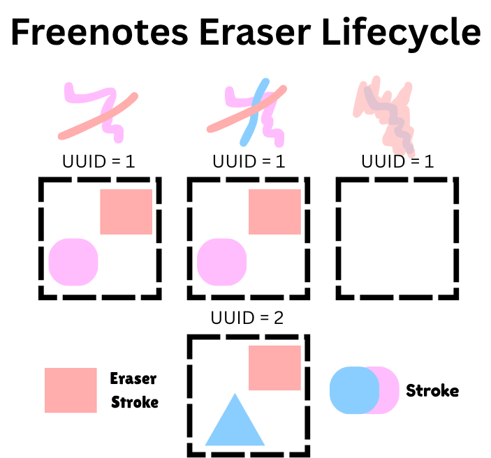
Freenotes handles stroke erasing in 2 primary ways:
- Entire stroke deleted
- Partial stroke deleted
The data structure containing eraser stroke data looks like this:
3 {
  1: "8EB54CB6-5BBD-4F94-B628-8E9C9E3481CD"
  2 {
    1 {
      1: "8EB54CB6-5BBD-4F94-B628-8E9C9E3481CD"
      2 {
        1: 1
        2: 377420543
      }
      3 {
        1: 0x3ff0000000000000
        4: 0x3ff0000000000000
      }
      4 {
        1: "15BA1FE2-22AC-4370-81ED-D79B6602183B"
        2 {
          1 {
            1: 0x40705c0338360178
            2: 0x403e59082a5b1a00
          }
          3 {
            1: 0x4002487100000000
            2: 0x4002487100000000
          }
          4: 0xbf98beaa80000000
        }
      ...
      5 {
        1: "57363165-BD86-49F6-9A04-3EA2C44B5786"
        2 {
          1: 101
        }
        3 {
          1: 0x3ff0000000000000
          4: 0x3ff0000000000000
        }
        4 {
          1: "BF9BCA51-959B-4123-AC9E-6128FA6FAC0F"
          2 {
            1 {
              1: 0x406fa3251751e1f4
              2: 0x40493b125eff6980
            }
            3 {
              1: 0x401469e640000000
              2: 0x401469e640000000
            }
            4: 0xbf8f712ce0000000
          }
From the Protobuf structure above, key components can be explained as follows:
-
field_4: Main pen stroke coordinates written initially by the user (pen color, stroke width, stylus pressure). Data infield_4is preserved 100% intact without discarding coordinates, as long as coordinates infield_4aren’t overlapped by eraser strokes (field_5). -
field_5: Path coordinates of the eraser tip, uniquely identified by Tool ID101(Eraser Brush). Tool ID 101 appears exclusively insidefield_5and never infield_2of main strokes.
Each Object
maintains its own independent field_4
and field_5
. If an eraser stroke passes across a stroke, the eraser coordinates are copied into field_5
of that stroke (passing 3 Strokes copies into field_5
across all 3 Strokes).
Lasso
In note-taking, another indispensable feature is Lasso. What is Lasso? Lasso, or Freeform Selection, allows selecting elements to perform actions like scaling or moving regardless of layers. Having read the Eraser section, you might better understand why eraser objects are stored separately per affected object rather than globally.
Because when moving or scaling objects, eraser paths move along with them, keeping stroke cuts intact. Before diving deeper, let’s examine the structure:
Before:
1: "0A7ACF32-9122-4274-A932-EE34D88740C2"
2: "EF7159AE-7834-41FC-B92A-AAD4F6B0DCF1"
3 {
  1: "5F7A6342-14E4-4005-8A7D-1EAA221DD7BF"
  2 {
    1 {
      1: "5F7A6342-14E4-4005-8A7D-1EAA221DD7BF"
      2 {
        1: 1
        2: 377420543
      }
      3 {
        1: 0x3ff0000000000000 # (double: 1.0)
        4: 0x3ff0000000000000 # (double: 1.0)
      }
      4 {
        1: "CBE801A9-59C1-4698-B9EC-61B12D3E0422"
        2 {
          1 {
            1: 0x4070da82b3c37a63 # (double: 269.6568865804606)
            2: 0x406886d5b4a4c882 # (double: 196.21308480620384)
          }
          3 {
            1: 0x4015d72cc0000000 # (double: 5.459999999999999)
            2: 0x4015d72cc0000000 # (double: 5.459999999999999)
          }
          4: 0xbf8c87e0c0000000 # (double: -0.013912320137023926)
        }
      ...
          3 {
            1: 0x4015d72cc0000000 # (double: 5.459999999999999)
            2: 0x4015d72cc0000000 # (double: 5.459999999999999)
          }
          4: 0x3fea4487c0000000 # (double: 0.8208653926849365)
        }
        3 {
          1: 1785729853
          2: 191121101
        }
        6: 4
      }
    }
    2: "EF7159AE-7834-41FC-B92A-AAD4F6B0DCF1"
    3: "EF7159AE-7834-41FC-B92A-AAD4F6B0DCF1"
  }
}
After:
1: "0A7ACF32-9122-4274-A932-EE34D88740C2"
2: "EF7159AE-7834-41FC-B92A-AAD4F6B0DCF1"
3 {
  1: "5F7A6342-14E4-4005-8A7D-1EAA221DD7BF"
  2 {
    1 {
      1: "5F7A6342-14E4-4005-8A7D-1EAA221DD7BF"
      2 {
        1: 2
        2: 377420416
      }
      3 {
        1: 0x3ff0000000000000 # (double: 1.0)
        4: 0x3ff0000000000000 # (double: 1.0)
        5: 0xc055e6da97516fe8 # (double: -87.60721867159892)
        6: 0x406008b4c3505ac0 # (double: 128.27200802891725)
      }
      4 {
        1: "32CD8D60-9A6D-4B91-AA07-3626A60C777B"
        2 {
          1 {
            1: 0x4074b0fb38a35ae8 # (double: 331.06142247294666)
            2: 0x406c994a7d67f8e0 # (double: 228.7888842988145)
          }
          3 {
            1: 0x402e16a260000000 # (double: 15.044208)
            2: 0x402e16a260000000 # (double: 15.044208)
          }
          4: 0xbf843c0d80000000 # (double: -0.0098801851272583)
        }
      ...
          3 {
            1: 0x402e16a260000000 # (double: 15.044208)
            2: 0x402e16a260000000 # (double: 15.044208)
          }
          4: 0x3fea4487c0000000 # (double: 0.8208653926849365)
        }
        3 {
          1: 1785729853
          2: 191121101
        }
        5: 0x400e28aba8559ead # (double: 3.7698668981162904)
        6: 4
      }
    }
    2: "64E033B5-37F4-4315-A4E2-D532689960F6"
    3: "64E033B5-37F4-4315-A4E2-D532689960F6"
  }
}
In Freenotes, when position is shifted, primary coordinates are not modified. Instead, an $X, Y$ offset is applied in the moved direction. Conversely, when resizing, coordinates are updated along with $X, Y$ radius values (line thickness), while recording the latest scale factor.
Highlighter
Based on our hypothesis observing Ballpoint Pen data blocks—that numbers in field_2
represent Hexadecimal colors and field_1
represents tip type—
we tested inspecting Highlighter strokes drawn on another page:
3 {
  1: "1494B805-9F85-4F16-B997-61C6C3D1A3A6"
  2 {
    1 {
      1: "1494B805-9F85-4F16-B997-61C6C3D1A3A6"
      2 {
        1: 2
        2: 1440180352 # #55D76990 Color Hex
      }
      ...
3 {
  1: "E53E9C9D-110F-433B-A86F-05863135D8AA"
  2 {
    1 {
      1: "E53E9C9D-110F-433B-A86F-05863135D8AA"
      2 {
        1: 2
        2: 4291768192  # #FFCF2F80 Color Hex
      }
Decoding yields semi-transparent highlighter yellow:
0xFF
CF
2F
80
- R (Red): 0xFF = 255
- G (Green): 0xCF = 207
- B (Blue): 0x2F = 47
- A (Alpha): 0x80 = 128 (approx. 50% opacity)
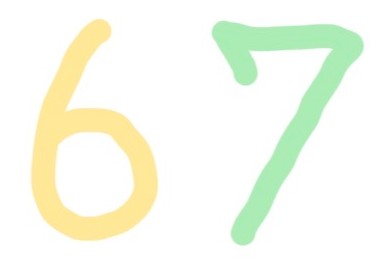
Read further in the next section.
[Highlight] Layered Rendering of Highlighter Colors
Having extracted semi-transparent highlighter colors (Alpha 50%), the next challenge is simulating highlighter strokes over text just like real highlighter pens in note apps, while managing RGBA Alpha down to RGB. Display pixels can only render opaque RGB colors per point; they cannot display true physical transparency. Alpha must be blended into the background to produce pure RGB before outputting to screen, and finally converted to standard monitor color space (sRGB).
In graphics engines, overlapping highlighter strokes cause blending between Source and Background layers.
Two compositing theories covered here are Multiply and Source Over—two among many Computer Graphics blending models chosen based on matching real Freenotes output (read more here). Color blending details are explored below.

This article uses the following notation throughout all equations:
- $C_s, c_s, \alpha_s$ : True color, Premultiplied color ($c_s = C_s \cdot \alpha_s$), and Alpha of Top layer (Source Layer)
- $C_b, c_b, \alpha_b$ : True color, Premultiplied color ($c_b = C_b \cdot \alpha_b$), and Alpha of Bottom layer (Backdrop Layer)
- $c_o, \alpha_o$ : Resulting Premultiplied color and total output Alpha
- $C_{\text{final}}$ : Final true color after removing Alpha ($C_{\text{final}} = \frac{c_o}{\alpha_o}$)
[Overlapping Highlighters] 1. Multiply Blending (Porter-Duff Multiply Blend Mode)
Instead of simply placing color on top, the system multiplies pixel color values between highlighter and base ink, following standard Computer Graphics blend modes.
Comparatively, this aligns with CAIRO_OPERATOR_MULTIPLY 12
Direct color multiplication formula (excluding Alpha):
$$c_o = c_s \cdot c_b$$Resulting overlay areas become darker than both inputs.
Example
Blending #55D76990 (Top color $c_s$) with #FFCF2F80 (Bottom color $c_b$) using Multiply Blend mode (RGB only, ignoring Alpha):
| Channel | Top Color ($c_s$) | Bottom Color ($c_b$) | Multiply ($c_o = c_s \cdot c_b$) | Result Hex |
|---|---|---|---|---|
| R (Red) | 0x55 (0.333) | 0xFF (1.000) | 0.333 × 1.000 = 0.333 | $(0.333/1)*255=85$ Round up = 0x55 |
| G (Green) | 0xD7 (0.843) | 0xCF (0.812) | 0.843 × 0.812 = 0.684 | $(0.684/1)*255=174$ Round up = 0xAE |
| B (Blue) | 0x69 (0.412) | 0x2F (0.184) | 0.412 × 0.184 = 0.076 | $(0.076/1)*255=19$ Round up = 0x13 |
Yielding blended color #55AE13
However, this formula ignores alpha values. Real applications must account for alpha values (0.0-1.0), modifying the formula as follows:
Pixel colors are processed in Premultiplied Alpha format (multiplying color $C$ by transparency $\alpha$ in advance: $c = C \cdot \alpha$).
Using Porter-Duff Source Over to calculate Cumulative Alpha ($\alpha_o$) across both layers can be visualized as a Venn Diagram:
Opacity set union formula:
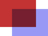
Substituting Alpha ($\alpha$) into the set equation:
$$ \alpha_o = \alpha_s + \alpha_b - (\alpha_s \cdot \alpha_b) $$$$ \alpha_o = \alpha_s + \alpha_b (1 - \alpha_s) $$Where:
- $\alpha_o$ [Total resulting opacity: Alpha Output at overlap point]
- $\alpha_s$ [Top layer opacity: Alpha Source of top stroke]
- $\alpha_b$ [Bottom layer opacity: Alpha Backdrop of lower stroke/background]
- $(1 - \alpha_s)$ [Remaining transparency ratio allowing backdrop light through]
Next, premultiplied colors ($c = C \cdot \alpha$) enter the Multiply blend equation, where overlapping terms cancel $\alpha$ variables, leaving:
$$ c_s \cdot c_b $$Combined with light passing through from both outer edges:
$$ c_o = (c_s \cdot c_b) + c_s \cdot (1 - \alpha_b) + c_b \cdot (1 - \alpha_s) $$Once calculated, premultiplied colors ($c_o$) convert back to standard color values for screen display by dividing by total Alpha ($\alpha_o$):
$$ C_{\text{final}} = \frac{c_o}{\alpha_o} $$Substituting top color #55D76990 ($\alpha_s = 0.565$) and bottom color #FFCF2F80 ($\alpha_b = 0.502$):
| Channel | Top Color ($c_s$) | Bottom Color ($c_b$) | Premultiplied Multiply ($c_o$) | Final Color after removing Alpha ($C_{\text{final}} = \frac{c_o}{\alpha_o}$) |
|---|---|---|---|---|
| R (Red) | $0.188$ | $0.502$ | $(0.188 \cdot 0.502) + 0.188(1-0.502) + 0.502(1-0.565) = \mathbf{0.406}$ | $\frac{0.406}{0.783} = 0.519 \rightarrow$ 0x84 |
| G (Green) | $0.476$ | $0.408$ | $(0.476 \cdot 0.408) + 0.476(1-0.502) + 0.408(1-0.565) = \mathbf{0.609}$ | $\frac{0.609}{0.783} = 0.777 \rightarrow$ 0xC6 |
| B (Blue) | $0.233$ | $0.092$ | $(0.233 \cdot 0.092) + 0.233(1-0.502) + 0.092(1-0.565) = \mathbf{0.178}$ | $\frac{0.178}{0.783} = 0.227 \rightarrow$ 0x3A |
| A (Alpha) | $0.565$ | $0.502$ | $\alpha_o = 0.565 + 0.502 \cdot (1 - 0.565) = \mathbf{0.783}$ | $0.783 \times 255 = 199 \rightarrow$ 0xC7 |
The final rendered color code appearing on screen is #84C63AC7
However, comparing this with our actual screenshot reveals colors do not match at all. Freenotes, Goodnotes, and note apps generally avoid Multiply blending because it darkens note text. Instead, they use the following blend formula.
[Overlapping Highlighters] 2. Source Over Blending (Porter-Duff Normal Blend Mode)
Normal Blending places “Source color” ($c_s$) over “Background color” ($c_b$), weighting by Source transparency ($\alpha_s$). Here is the rendered image using Normal Blending (Source Over)13 with original colors and transparency:
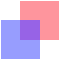
| Channel | Top Color ($c_s$) | Bottom Color ($c_b$) | Premultiplied Source Over ($c_o = c_s + c_b(1-\alpha_s)$) | Final Color after removing Alpha ($C_{\text{final}} = \frac{c_o}{\alpha_o}$) |
|---|---|---|---|---|
| R (Red) | $0.188$ | $0.502$ | $0.188 + 0.502 \cdot (1 - 0.565) = \mathbf{0.406}$ | $\frac{0.406}{0.783} = 0.519 \rightarrow$ 0x84 |
| G (Green) | $0.476$ | $0.408$ | $0.476 + 0.408 \cdot (1 - 0.565) = \mathbf{0.653}$ | $\frac{0.653}{0.783} = 0.834 \rightarrow$ 0xD5 |
| B (Blue) | $0.233$ | $0.092$ | $0.233 + 0.092 \cdot (1 - 0.565) = \mathbf{0.273}$ | $\frac{0.273}{0.783} = 0.349 \rightarrow$ 0x59 |
| A (Alpha) | $0.565$ | $0.502$ | $\alpha_o = 0.565 + 0.502 \cdot (1 - 0.565) = \mathbf{0.783}$ | $0.783 \times 255 = 199 \rightarrow$ 0xC7 |
Summary of final color code: #84D559C7 (Pastel light green)
[Overlapping Highlighters] Key Insight: Why Source Over Instead of Multiply?
Having calculated both highlighter overlap formulas, which formula is better?
Neither is inherently better; both are valid engineering/design decisions answering different user needs. Developers choose based on trade-offs:
-
Multiply: Colors darken with every overlap, suitable for artwork showing layer density (standard painting apps).
-
Source Over: Base ink color remains unchanged regardless of highlighter layer count, because Source Over weights heavily by top-layer highlighter alpha rather than accumulating darkness.
For note-taking apps like Freenotes, Source-Over is ideal because highlighting emphasizes text without altering user handwriting colors. With Multiply, multiple highlighter strokes would progressively black out handwriting.
Removing Alpha from Color Codes
Even though this color is correct theoretically, sampling color with a browser Color Picker shows values still don’t match.
This is because our calculations haven’t accounted for the bottom-most layer: white paper (#FFFFFF), which browsers automatically compute.
To get true screen values, we must calculate Screen Color ($C_{\text{screen}}$), since monitor RGB pixels emit 100% light. Applying Source Over over white paper ($C_{\text{paper}} = 1.0$):
$$C_{\text{screen}} = c_o + C_{\text{paper}} \cdot (1 - \alpha_o)$$Comparing with blank white paper (#FFFFFF) where $C_{\text{paper}} = 1.0$:
Substituting $c_o = C_{\text{final}} \cdot \alpha_o$ into the equation:
$$C_{\text{screen}} = C_{\text{final}} \cdot \alpha_o + (1 - \alpha_o)$$Rearranging yields the formula for actual screen color ($C_{\text{screen}}$):
$${C_{\text{screen}} = c_o + (1 - \alpha_o)}$$Converting Scale to 8-Bit Pixels ($0 - 255$)
Since display pixels and browser Color Pickers store each RGB channel as 8-bit values (8 bits per channel) between $0$ and $255$ (0xFF), we multiply $C_{\text{screen}}$ ($0.0 - 1.0$) by $255$:
Substituting $c_o$ and $\alpha_o = 0.783$ (white paper light passing through $1 - 0.783 = 0.217$):
| Channel | Premultiplied Color ($c_o \times 255$) | White paper light passing through ($(1 - \alpha_o) \times 255$) | Total pixel value on screen ($C_{\text{screen}} \times 255$) | Hex |
|---|---|---|---|---|
| R (Red) | $0.406 \times 255 = 103.5$ | $0.217 \times 255 = 55.3$ | $103.5 + 55.3 = \mathbf{158.8} \approx 159$ | 0x9F |
| G (Green) | $0.653 \times 255 = 166.5$ | $0.217 \times 255 = 55.3$ | $166.5 + 55.3 = \mathbf{221.8} \approx 222$ | 0xDE |
| B (Blue) | $0.273 \times 255 = 69.6$ | $0.217 \times 255 = 55.3$ | $69.6 + 55.3 = \mathbf{124.9} \approx 125$ | 0x7D |
Screen output color code is #9FDE7D, which may still slightly differ from Browser Color Pickers (e.g. #A8DF7E). This occurs because modern displays use sRGB (Standard RGB) color space rather than linear RGB ($C_{\text{screen}}$). Human vision is more sensitive to dark tones, so sRGB compresses Linear RGB with a standard Gamma of $2.2$.
Calculating Colors for Displays
As mentioned, after alpha blending and alpha removal, linear RGB ($C_{\text{screen}}$) is still insufficient for sRGB displays.
We must convert Linear RGB ($C_{\text{screen}}$) to sRGB ($C_{\text{sRGB}}$) via Gamma Correction ($\gamma = 2.2$) 6
Converting Linear RGB to sRGB
Per IEC 61966-2-17, converting linear color $C_{\text{screen}}$ ($0.0 - 1.0$) to $C_{\text{sRGB}}$ is calculated by:
$$C_{\text{sRGB}} = \begin{cases} 12.92 \cdot C_{\text{screen}}, & C_{\text{screen}} \le 0.0031308 \\ 1.055 \cdot C_{\text{screen}}^{1/2.2} - 0.055, & C_{\text{screen}} > 0.0031308 \end{cases}$$Or estimated via Gamma Power Law:
$$C_{\text{sRGB}} \approx \left( C_{\text{screen}} \right)^{\frac{1}{2.2}}$$| Channel | Hex Value | Linear Value ($C_{\text{screen}} = \text{Hex}/255$) | After Gamma $2.2$ ($C_{\text{sRGB}} = C_{\text{screen}}^{1/2.2}$) | Total pixel value on screen ($C_{\text{sRGB}} \cdot 255$) | Hex |
|---|---|---|---|---|---|
| R (Red) | 0x9F (159) | 159 / 255 = 0.623529 | (0.623529)^0.4545 = 0.658764 | $0.658764 * 255 = \mathbf{167.98} \approx 168 $ | 0xA8 |
| G (Green) | 0xDE (222) | 222 / 255 = 0.870588 | (0.870588)^0.4545 = 0.938927 | $0.938927 * 255 = \mathbf{223.42} \approx 223$ | 0xDF |
| B (Blue) | 0x7D (125) | 125 / 255 = 0.490196 | (0.490196)^0.4545 = 0.494164 | $0.494164 * 255 = \mathbf{126.01} \approx 126 $ | 0x7E |
Ultimately, the color code equals #A8DF7E, resulting from two Source Over blend passes:
- First pass against the underlying stroke
- Second pass against white paper (Background)
followed by alpha compression onto RGB without quality loss, and finally converting Linear RGB to sRGB to match actual screen displays.
Sampling overlapping colors with a browser Color Picker now yields exact matching values.
Calculating Pen Stroke Width
Stepping back briefly… we haven’t discussed stroke width calculation in Freenotes. Freenotes has a single UI parameter for line width: Thickness, ranging from $1.0 - 15.0$.
Decoded Protobuf fields store values for $1.0$ and $15.0$ as follows:
4 {
  1: "C170DC0C-03D6-4826-A674-030C1F37E9A0"
  2 {
    1 {
      1: 0x4077c9d0ab6541b0 # (double: 380.613445)
      2: 0x405c7d60c9f44148 # (double: 113.959033)
    }
    3 {
      1: 0x4002da8d40000000 # (double: 2.356715)
      2: 0x4002da8d40000000 # (double: 2.356715)
    }
    4: 0xbf8c87e0c0000000 # (double: -0.013912320137023926)
  }
4 {
1: "031183C5-74C2-4061-B2E7-012C73A3AE81"
2 {
1 {
1: 0x40777122f0175b79 # (double: 375.07103)
2: 0x405a52287e36fab0 # (double: 105.283721)
}
3 {
1: 0x401d672300000000 # (double: 7.350719)
2: 0x401d672300000000 # (double: 7.350719)
}
4: 0xbf8c87e0c0000000 # (double: -0.013912320137023926)
}Converting Freenotes Weight -> Point Size (pt)
Adjusting pen thickness in Freenotes UI and inspecting decoded Protobuf values reveals recorded Weight values aren’t saved directly in Points ($pt$), but undergo transformation.
Observing two baseline reference points at minimum ($T = 1.0$) and maximum ($T = 15.0$) thickness:
- Thickness $1.0$ pt $\rightarrow$ Protobuf value:
2.356715 - Thickness $15.0$ pt $\rightarrow$ Protobuf value:
7.350719
Testing a linear relationship hypothesis:
$$ f(T) = \alpha \cdot T + \beta = V $$Where $T$ is Thickness in pt and $V$ is recorded Protobuf weight.
Substituting test points into equations:
$$ f(1.0) = 1.0 \alpha + \beta = 2.356715 \quad \text{--- (1)} $$$$ f(15.0) = 15.0 \alpha + \beta = 7.350719 \quad \text{--- (2)} $$
Subtracting equation $(2) - (1)$ to eliminate $\beta$:
$$ 14\alpha = 7.350719 - 2.356715 $$$$ 14\alpha = 4.994004 $$
$$ \mathbf{\alpha = \frac{4.994004}{14} = 0.356714571 \approx 0.356715} $$
Substituting $\alpha \approx 0.356715$ back into $(1)$:
$$ (0.356715 \times 1.0) + \beta = 2.356715 $$$$ \mathbf{\beta = 2.356715 - 0.356715 = 2.000000} $$
Yielding the complete conversion equation from $pt$ to recorded file weight:
$$ V = f(T) = 0.356715 \cdot T + 2.00 $$To decode back from Protobuf values to point size ($pt$):
$$ T = \frac{V - 2.00}{0.356715} \quad \text{(pt)} $$Testing and Validating the Formula
Testing this formula against other size values outside baseline points confirms linear coverage:
1. Pen size $7.3$ pt
- Calculated recorded value ($V$): $$V = 2.00 + (0.356715 \times 7.3) = 4.6040195$$
- Actual value found in Protobuf file:
4.604017(Error of $0.0000025$) - Decoding back: $$T = \frac{4.604017 - 2.00}{0.356715} = \frac{2.604017}{0.356715} \approx 7.300004 \text{ pt}$$
2. Highlighter size $30.0$ pt
- Calculated recorded value ($V$): $$V = 2.00 + (0.356715 \times 30.0) = 12.70145$$
- Actual value found in Protobuf file:
12.701439 - Decoding back: $$T = \frac{12.701439 - 2.00}{0.356715} = \frac{10.701439}{0.356715} \approx 29.999969 \approx 30.0 \text{ pt}$$
The linear formula $V = 0.356715 \cdot T + 2.00$ converts bidirectionally with nearly 100% accuracy. The constant $\beta = 2.00$ is assumed to be Freenotes' Base Offset Radius.
Multi-Pass Z-Layering
In actual usage, users write black text first and highlight over it later. If rendered in chronological order (Time-series), highlighter strokes would sit on top of ink lines. Why not use layers like Krita?
Because this isn’t Krita. Krita isn’t designed as a note app. Although Freenotes supports layers, average note-takers don’t constantly switch active layers.
As a note app, the optimal solution is re-ordering Z-Passes based on tool tip type (Highlighter = 2).
The reverse-engineered rendering system operates in 2 passes (2-Pass Render Loop):
1. Pass 1 (Lower Z-Pass - Highlighter):
Scans FNPages stroke arrays for tool_type == 2 (Highlighter), rendering them onto the canvas first as the lower layer beneath text.
2. Pass 2 (Upper Z-Pass - Ink Stroke):
Scans strokes with tool_type != 2 (Ballpoint, Fountain, Pencil), rendering them on top so black handwriting remains sharp and unobscured.
# Reverse-Engineered Renderer
def render_page_strokes_with_z_order(ctx, page_strokes):
    # Pass 1: Draw all highlighter strokes on the lower layer first
    for stroke in page_strokes:
        if stroke.tool_type == 2:  # Highlighter
            draw_bezier_path(ctx, stroke.points, stroke.color, stroke.width)

    # Pass 2: Draw regular ink strokes on top of the upper layer
    for stroke in page_strokes:
        if stroke.tool_type != 2:  # Regular Pens
            draw_bezier_path(ctx, stroke.points, stroke.color, stroke.width)
Eraser Path Integration
On every draw pass, the engine checks eraser paths (field_5
/ Eraser Tool ID 101), using Clear Operator mode (cairo.OPERATOR_CLEAR) to slice strokes before compositing onto white paper (#FFFFFF).
[Eraser] Designing an Eraser Engine
Note: What we are doing here is comparing point-to-point, whereas in reality vector line segment overlap should be evaluated, as strokes consist of thick line segments rather than isolated points. Point-only detection causes unnatural stroke breaks.
First, let’s review Eraser object structures:
5 {
  1: "E76432F0-7870-4F87-9C95-1C7A826E097C"
  2 {
    1: 101
  }
  3 {
    1: 0x3ff0000000000000 # 4607182418800017408 (double: 1.0)
    4: 0x3ff0000000000000 # 4607182418800017408 (double: 1.0)
  }
  4 {
    1: "6D1279C6-1FDC-467F-8141-2B43C495F640"
    2 {
      1 {
        1: 0x4067026487fe2766 # 4640680571830151014 (double: 184.07674296048283)
        2: 0x4077b98267580d10 # 4645204090968083728 (double: 379.5975656105)
      }
      3 {
        1: 0x401469e640000000 # 4617332999552237568 (double: 5.103416442871094)
        2: 0x401469e640000000 # 4617332999552237568 (double: 5.103416442871094)
      }
      4: 0xbf857f6de0000000 # 13800520563544645632 (double: -0.010496958158910275)
    }
The Protobuf structure of an eraser tip is virtually identical to pen objects, allowing identical coordinate and width decoding.
Notice in line weight fields:
3 {
  1: 0x401469e640000000 # 4617332999552237568 (double: 5.103416442871094)
  2: 0x401469e640000000 # 4617332999552237568 (double: 5.103416442871094)
}
Values 5.103416442871094 in fields 1 and 2 represent Start Weight ($V_{start}$) and End Weight ($V_{end}$).
1. Decoding Eraser Tip Width to UI Thickness (pt)
$$T = \frac{V - 2.00}{0.356715}$$$$T = \frac{5.103416442871094 - 2.00}{0.356715} = \frac{3.103416442871094}{0.356715} \approx \mathbf{8.70\text{ pt}}$$Applying Weight $V = 5.10341644$ to our decoding formula:
The eraser tip size was set to $8.70\text{ pt}$ in Freenotes.
2. Geometric Overlap Detection
$$d(P, E) = \sqrt{(x_p - x_e)^2 + (y_p - y_e)^2}$$When dragging an eraser at $E = (x_e, y_e)$ with thickness $T_e = 8.70\text{ pt}$ (erasing radius $R_e \approx 4.35\text{ pt}$), 2D Euclidean Distance is calculated to original ink point $P = (x_p, y_p)$ with ink radius $r_p$:
$$d(P, E) \le R_e + r_p$$Overlap Condition:
- If true ($d \le R_e + r_p$): Eraser boundary overlaps ink stroke; system splits stroke or deletes segment.
Eraser Collision Calculation Example
Given:
-
$P = (10, 15)$ [Original ink coordinate]
-
$r_p = 2.0\text{ pt}$ [Original ink radius]
-
$E = (14, 18)$ [Eraser tip coordinate]
-
$R_e = 4.35\text{ pt}$ [Eraser tip radius $8.70 / 2$]
- Calculate Euclidean distance ($d$) between ink $P(10,15)$ and eraser $E(14,18)$:
- Calculate combined radius sum ($R_e + r_p$):
- Check collision condition ($d \le R_e + r_p$):
Distance $5.0\text{ pt}$ is less than radius sum $6.35\text{ pt}$, confirming eraser overlap.
[Lasso] Transformations
$$x' = A x + b$$All spatial transformations stem from the linear affine transformation equation:
Where:
-
$x$ is original coordinate vector
-
$x'$ is transformed coordinate vector
-
$A$ is linear transformation matrix (rotation, scaling, shear, reflection)
-
$b$ is translation vector
Matrix representation in 2D ($3 \times 3$):
$$ \begin{bmatrix} x' \\ y' \\ 1 \end{bmatrix} = \begin{bmatrix} a & b & e \\ c & d & f \\ 0 & 0 & 1 \end{bmatrix} \begin{bmatrix} x \\ y \\ 1 \end{bmatrix} $$Translation
Translation moves stroke objects when dragging with Lasso Tool.
In vector storage, Freenotes doesn’t recompute primary stroke coordinates; it applies Matrix Offset:
$$ T(t_x, t_y) = \begin{bmatrix} 1 & 0 & t_x \\ 0 & 1 & t_y \\ 0 & 0 & 1 \end{bmatrix} $$Combining with the initial equation, this transforms to:
$$ \begin{bmatrix} x' \\ y' \\ 1 \end{bmatrix} = \begin{bmatrix} 1 & 0 & t_x \\ 0 & 1 & t_y \\ 0 & 0 & 1 \end{bmatrix} \begin{bmatrix} x \\ y \\ 1 \end{bmatrix} = \begin{bmatrix} x + t_x \\ y + t_y \\ 1 \end{bmatrix} $$Example
Given:
- $x$ representing x-axis equals $269.65$
- $y$ representing y-axis equals $196.21$
- $t_x$ representing x-axis shift equals $-87.60$
- $t_y$ representing y-axis shift equals $128.27$
Substituting values:
$$ \begin{bmatrix} x' \\ y' \\ 1 \end{bmatrix} = \begin{bmatrix} 1 & 0 & -87.60 \\ 0 & 1 & 128.27 \\ 0 & 0 & 1 \end{bmatrix} \begin{bmatrix} 269.65 \\ 196.21 \\ 1 \end{bmatrix} $$$$ \begin{bmatrix} x' \\ y' \\ 1 \end{bmatrix} = \begin{bmatrix} 269.65 + (-87.60) \\ 196.21 + 128.27 \\ 1 \end{bmatrix} = \begin{bmatrix} \mathbf{182.05} \\ \mathbf{324.48} \\ 1 \end{bmatrix} $$Screen position evaluates to $(182.05, 324.48)$, while internal stored coordinates remain $(269.65, 196.21)$.
Scaling
Scaling resizes along X by factor $s_x$ and Y by factor $s_y$:
When scaling in Freenotes, primary coordinates are updated to match the new scale, unlike translation which preserves original values.
$$ S(s_x, s_y) = \begin{bmatrix} s_x & 0 & 0 \\ 0 & s_y & 0 \\ 0 & 0 & 1 \end{bmatrix} $$Combining with general coordinate transformation equations yields:
$$ \begin{bmatrix} x' \\ y' \\ 1 \end{bmatrix} = \begin{bmatrix} s_x & 0 & 0 \\ 0 & s_y & 0 \\ 0 & 0 & 1 \end{bmatrix} \begin{bmatrix} x \\ y \\ 1 \end{bmatrix} = \begin{bmatrix} s_x \cdot x \\ s_y \cdot y \\ 1 \end{bmatrix} $$Scaling in note apps pivots around the Bounding Box Center ($C_x, C_y$) rather than $(0,0)$ to maintain object position:
$$ \begin{bmatrix} x' \\ y' \\ 1 \end{bmatrix} = \begin{bmatrix} 1 & 0 & C_x \\ 0 & 1 & C_y \\ 0 & 0 & 1 \end{bmatrix} \begin{bmatrix} s_x & 0 & 0 \\ 0 & s_y & 0 \\ 0 & 0 & 1 \end{bmatrix} \begin{bmatrix} 1 & 0 & -C_x \\ 0 & 1 & -C_y \\ 0 & 0 & 1 \end{bmatrix} \begin{bmatrix} x \\ y \\ 1 \end{bmatrix} $$$$ \begin{bmatrix} x' \\ y' \\ 1 \end{bmatrix} = \begin{bmatrix} s_x & 0 & C_x(1 - s_x) \\ 0 & s_y & C_y(1 - s_y) \\ 0 & 0 & 1 \end{bmatrix} \begin{bmatrix} x \\ y \\ 1 \end{bmatrix} $$$$ x' = C_x + s_x \cdot (x - C_x) $$$$ y' = C_y + s_y \cdot (y - C_y) $$Example
Given:
- $x$ representing x-axis equals $269.65$
- $y$ representing y-axis equals $196.21$
- $s_x$ representing x-axis scale factor equals $3.76$
- $s_y$ representing y-axis scale factor equals $3.76$
Substituting values:
$$ x' = 247.1983 + 3.769859 \times (269.656910 - 247.1983) = \mathbf{331.870204\text{ px}} $$$$ y' = 250.3054 + 3.769859 \times (196.213587 - 250.3054) = \mathbf{46.387123\text{ px}} $$Yielding $(331.870204, 46.387123)$, resulting from 3.76x scaling centered on itself.
Rotation
Rotation rotates objects by an angle without storing legacy coordinates, replacing values directly.
Rotation matrix around center pivot point ($C_x, C_y$):
$$ {\begin{bmatrix}\cos(\theta )&-\sin(\theta )&0\\\sin(\theta )&\cos(\theta )&0\\0&0&1\end{bmatrix}} $$Scaling and rotation pivot around the Bounding Box Center ($C_x, C_y$):
$$ \begin{bmatrix} x' \\ y' \\ 1 \end{bmatrix} = \begin{bmatrix} 1 & 0 & C_x \\ 0 & 1 & C_y \\ 0 & 0 & 1 \end{bmatrix} \begin{bmatrix} \cos\theta & -\sin\theta & 0 \\ \sin\theta & \cos\theta & 0 \\ 0 & 0 & 1 \end{bmatrix} \begin{bmatrix} 1 & 0 & -C_x \\ 0 & 1 & -C_y \\ 0 & 0 & 1 \end{bmatrix} \begin{bmatrix} x \\ y \\ 1 \end{bmatrix} $$$$ \begin{bmatrix} x' \\ y' \\ 1 \end{bmatrix} = \begin{bmatrix} \cos\theta & -\sin\theta & C_x(1 - \cos\theta) + C_y\sin\theta \\ \sin\theta & \cos\theta & C_y(1 - \cos\theta) - C_x\sin\theta \\ 0 & 0 & 1 \end{bmatrix} \begin{bmatrix} x \\ y \\ 1 \end{bmatrix} $$$$ x' = C_x + (x - C_x)\cos\theta - (y - C_y)\sin\theta $$$$ y' = C_y + (x - C_x)\sin\theta + (y - C_y)\cos\theta $$
Example
Given:
- $x$ representing x-axis equals $268.31$
- $y$ representing y-axis equals $144.09$
- $C_x$ representing center point x-axis equals $282.25$
- $C_y$ representing center point y-axis equals $137.64$
- $\theta$ representing rotation angle (counterclockwise) equals $90^\circ$ ($\cos 90^\circ = 0, \sin 90^\circ = 1$)
Substituting values:
$$ x' = 282.2467 + (268.3091 - 282.2467)\cos 90^\circ - (144.0901 - 137.6390)\sin 90^\circ $$$$ = \mathbf{275.7956\text{ px}} $$$$ y' = 137.6390 + (268.3091 - 282.2467)\sin 90^\circ + (144.0901 - 137.6390)\cos 90^\circ $$$$ = \mathbf{123.7014\text{ px}} $$
Yielding $(275.7956, 123.7014)$, resulting from 90° rotation centered on itself.
Conclusion
After writing such a lengthy post, what is the conclusion? Building note-taking apps is ridiculously hard! haha
Regardless, this is the charm of Vector Graphics. Throughout all the operations we performed, not a single detail of the stroke was degraded—whether layering color, rotating, scaling, or anything else, the result remains crisp vector strokes as always.
There isn’t much left to say in this final section since I’ve written so much already.
So I got my agent to take this entire article as a prompt to build a simple WebGL Note-taking app to try out. Have fun testing it xoxo
This is the longest article I’ve ever written in my life (next time I’ll split it into parts).
If there are any errors or anything you’d like to add, feel free to leave comments and feedback 🥰
Appendix: Raw Protobuf Decoded Dumps
[BOX] A. document.dat (Full Raw Decoded Dump) [ CLICK TO UNBOX ] [ CLICK TO CLOSE ]
1: 2
2: "915CB187-E62E-439E-AD9B-DC50DA3AAC13"
4 {
  1 {
    1: "AA553773-6919-4ECA-B97F-DAA2ADE15E06"
    5 {
      1: "2018E179-78B1-4CF2-A8D5-1E002442D853"
      2: 1
      4 {
        1: 1
        3 {
          1: "A998661F-669C-4F73-8D21-21E16BF1496C"
          2: "2F8DA175-4F19-4ADA-9FD2-B2369CE08F77" # REF: PDFs/<uuid>.pdf
          4: "common1_A3_5_vertical_color5"
          6: 1
          7: 3068264191
          9: 1
          10: "common_cover_identifier_38"
        }
      }
    }
    11 {
      1: 1785397999
      2: 501024961
    }
  }
  1 {
    1: "1AF3A213-07F5-45B4-BA87-E63E7B9AE6C9"
    3: 1
    5 {
      1: "A9BB4458-0053-4953-8CE4-AD21FFE7A7DB"
      3 {
        2: 5
        3: 4294967295
        4: 3166485759
        5: 1
      }
    }
    6: "3C892967-BC80-4C5F-B384-FB2045DEC9CA" # REF: FNPages/<uuid>.dat
    8: "D0E31896-FAE8-460B-A9F8-69909A199688" # REF: OCR_v3/en-US/<uuid>/content.json
    11 {
      1: 1785397999
      2: 484833956
    }
  }
  1 {
    1: "D7341019-D335-43EB-BBE8-B7B59D31303E"
    3: 2
    5 {
      1: "A9BB4458-0053-4953-8CE4-AD21FFE7A7DB"
      3 {
        2: 5
        3: 4294967295
        4: 3166485759
        5: 1
      }
    }
    11 {
      1: 1785397999
      2: 484909058
    }
  }
  2 {
    1: "2F8DA175-4F19-4ADA-9FD2-B2369CE08F77" # REF: PDFs/<uuid>.pdf
    2: "AA553773-6919-4ECA-B97F-DAA2ADE15E06"
    3 {
      1: 0
      2 {
        2: "AA553773-6919-4ECA-B97F-DAA2ADE15E06"
      }
    }
  }
  5: 1
}
6 {
  1: 1785397999
  2: 484794140
}
7: 2
Document_uuid Page_uuid Pdf_uuid FNPages_uuid OCR_uuid
[BOX] B. FNPages/3C892967-BC80-4C5F-B384-FB2045DEC9CA.dat (Full Raw Decoded Dump) [ CLICK TO UNBOX ] [ CLICK TO CLOSE ]
1: "3C892967-BC80-4C5F-B384-FB2045DEC9CA"
2: "1AF3A213-07F5-45B4-BA87-E63E7B9AE6C9"
3 {
  1: "54C99B69-BB82-4936-A855-9354BAE8C45B"
  2 {
    1 {
      1: "54C99B69-BB82-4936-A855-9354BAE8C45B"
      2 {
        1: 1
        2: 2377619967         # #8DB799FF Color Hex
      }
      3 {
        1: 0x3ff0000000000000 # 4607182418800017408 (double: 1.0)
        4: 0x3ff0000000000000 # 4607182418800017408 (double: 1.0)
      }
      4 {
        1: "2A59792B-ED5F-447D-9680-E0D230B07858"
        2 {
          1 {
            1: 0x4064a0b4eb000000 # 4640028243290628096 (double: 165.02208614349365)
            2: 0x4064a842f20b1378 # 4640036553818313592 (double: 165.2581723947078)
          }
          3 {
            1: 0x4002917f20000000 # 4612349070775910400 (double: 2.321044921875)
            2: 0x4002917f20000000 # 4612349070775910400 (double: 2.321044921875)
          }
          4: 0xbf90647fe0000000 # 13803606670868217856 (double: -0.016008377075195312)
        }
        2 {
          1 {
            1: 0x4064f20362e80000 # 4640117703550238720 (double: 167.56289291381836)
            2: 0x4064b466bc170e50 # 4640049909204094544 (double: 165.6375402379781)
          }
          3 {
            1: 0x4002917f20000000 # 4612349070775910400 (double: 2.321044921875)
            2: 0x4002917f20000000 # 4612349070775910400 (double: 2.321044921875)
          }
          4: 0x3f74721920000000 # 4572412853765111808 (double: 0.004991650581359863)
        }
        2 {
          1 {
            1: 0x4065bd4797f80000 # 4640343336494628864 (double: 173.91500091552734)
            2: 0x4064d0e753d760a0 # 4640081297780039840 (double: 166.5282381283321)
          }
          3 {
            1: 0x4002917f20000000 # 4612349070775910400 (double: 2.321044921875)
            2: 0x4002917f20000000 # 4612349070775910400 (double: 2.321044921875)
          }
          4: 0x3f9684f900000000 # 4581987541655027712 (double: 0.021991610527038574)
        }
        2 {
          1 {
            1: 0x4066cec3f6600000 # 4640644342516350976 (double: 182.46142482757568)
            2: 0x4064ece0c4a43de8 # 4640112048504028648 (double: 167.43369062638842)
          }
          3 {
            1: 0x4002917f20000000 # 4612349070775910400 (double: 2.321044921875)
            2: 0x4002917f20000000 # 4612349070775910400 (double: 2.321044921875)
          }
          4: 0x3fa373a200000000 # 4585623049581920256 (double: 0.037991583347320557)
        }
        2 {
          1 {
            1: 0x4067f1257c000000 # 4640963500353159168 (double: 191.53582382202148)
            2: 0x4064f7f640c94ea4 # 4640124239853760164 (double: 167.74880983636504)
          }
          3 {
            1: 0x4002917f20000000 # 4612349070775910400 (double: 2.321044921875)
            2: 0x4002917f20000000 # 4612349070775910400 (double: 2.321044921875)
          }
          4: 0x3faa1b9300000000 # 4587494541332611072 (double: 0.05100008845329285)
        }
        2 {
          1 {
            1: 0x406a7b1248100000 # 4641678170286358528 (double: 211.84600067138672)
            2: 0x4064d5a764798c64 # 4640086522616122468 (double: 166.6766835154381)
          }
          3 {
            1: 0x4002917f20000000 # 4612349070775910400 (double: 2.321044921875)
            2: 0x4002917f20000000 # 4612349070775910400 (double: 2.321044921875)
          }
          4: 0x3fb26e0b00000000 # 4589836932400906240 (double: 0.07200008630752563)
        }
        3 {
          1: 1785398005
          2: 835236073
        }
        6: 4
      }
    }
    2: "1AF3A213-07F5-45B4-BA87-E63E7B9AE6C9"
    3: "1AF3A213-07F5-45B4-BA87-E63E7B9AE6C9"
  }
}
Document_uuid Page_uuid Pdf_uuid FNPages_uuid OCR_uuid
[BOX] C. PDFs/Layout.dat (Full Raw Decoded Dump) [ CLICK TO UNBOX ] [ CLICK TO CLOSE ]
1: "915CB187-E62E-439E-AD9B-DC50DA3AAC13"
2: 0x4082980000000000 # 4648439126305964032 (double: 595.0)
3 {
  1 {
    1: 0x4082980000000000 # 4648439126305964032 (double: 595.0)
    2: 0x408a4cf81852b2c6 # 4650644485586170566 (double: 841.6211242675781)
  }
  2: 0x3fe69ce2344b66c4 # 4604539121650330308 (double: 0.7066507339477539)
  3: ""
  5: "AA553773-6919-4ECA-B97F-DAA2ADE15E06"
}
3 {
  1 {
    1: 0x4082980000000000 # 4648439126305964032 (double: 595.0)
    2: 0x408a500000000000 # 4650647820000000000 (double: 842.0)
  }
  2: 0x3ff0000000000000 # 4607182418800017408 (double: 1.0)
  3 {
    2: 0x408a4cf81852b2c6 # 4650644485586170566 (double: 841.6211242675781)
  }
  4: 1
  5: "1AF3A213-07F5-45B4-BA87-E63E7B9AE6C9"
}
3 {
  1 {
    1: 0x4082980000000000 # 4648439126305964032 (double: 595.0)
    2: 0x408a500000000000 # 4650647820000000000 (double: 842.0)
  }
  2: 0x3ff0000000000000 # 4607182418800017408 (double: 1.0)
  3 {
    2: 0x409a4e7c0c295963 # 4655022137682221411 (double: 1683.6211242675781)
  }
  4: 2
  5: "D7341019-D335-43EB-BBE8-B7B59D31303E"
}
4 {
  2: "AA553773-6919-4ECA-B97F-DAA2ADE15E06"
  2: "1AF3A213-07F5-45B4-BA87-E63E7B9AE6C9"
  2: "D7341019-D335-43EB-BBE8-B7B59D31303E"
}
Document_uuid Page_uuid Pdf_uuid FNPages_uuid OCR_uuid
-
https://docs.kanzi.com/3.9.1/en/working-with/2d-content/blending-2d-nodes.html#alpha-premultiplied ↩︎
-
https://www.w3.org/TR/compositing-1/#porterduffcompositingoperators_srcover ↩︎ ↩︎
-
https://webgl.brown37.net/12_advanced_rendering/05_color_blending.html ↩︎
-
https://cdn.standards.iteh.ai/samples/10795/ae461684569b40bbbb2d9a22b1047f05/IEC-61966-2-1-1999-AMD1-2003.pdf The full document are behind a huge sum paywall, legally obtain it at your very owned risk ↩︎
-
https://medium.com/@tomforsyth/the-srgb-learning-curve-773b7f68cf7a ↩︎
-
https://en.wikipedia.org/wiki/Affine_transformation#Representation ↩︎
-
https://en.wikipedia.org/wiki/Affine_transformation#Augmented_matrix ↩︎
-
https://en.wikipedia.org/wiki/Affine_transformation#Image_transformation ↩︎ ↩︎ ↩︎
Comments